Create maps on RStudio with the leaflet() package

Do you need to create interactive maps for your spatial data analysis? Look no further! With RStudio and the leaflet package, you can easily create interactive maps to visualize your spatial data simply and beautifully. In this article, we will show you how to create an interactive map using the leaflet package for RStudio. And to give you a taste, we will give you an example of a map that shows the main monuments of France. So, are you ready to explore spatial data? Let’s go !

Introduction to the leaflet package

Firstly, what is Leaflet? Leaflet is a mapping package for RStudio that allows you to create interactive and dynamic maps. It uses the Leaflet JavaScript library to create interactive maps in RStudio. Maps can be zoomed and moved, and data can be represented as markers, circles, polygons, etc.

The leaflet package is easy to use and provides functions for creating basic maps, adding markers, circles, polygons and tile layers. In addition, it is possible to customize the appearance of the maps using CSS.

We will use to image this article a public dataset available on the french website data.gouv.fr called “Liste des coordonnées GPS des monuments nationaux” (List of GPS coordinates of national monuments) . I recommend you to download it on your computer if you want to replicate the steps, or simply to use one of your dataset.

Step 1: Installation and loading of the leaflet package

The first step is to install the leaflet package. Open RStudio and run the following command:

install.packages("leaflet")
codelibrary(leaflet)
library(dplyr)

Step 2: Loading the data

We will now load our data to display the markers on the map. After downloading the National Monuments file in CSV format that contains the names, geographic coordinates and descriptions of some of the monuments in Paris, we will load it into RStudio. Since our file is a csv separated by a semi-colon “;”, I use the “read.csv2()” function.

monuments <- read.csv2("votre-chemin-dacces/liste-coordonnees-gps-des-monuments.csv", stringsAsFactors = FALSE)
head(monuments, n=5)

 monument_id             id                                                       name                          latitude                        longitude
1          58             103706     Abbaye de Beaulieu-en-Rouergue                   44.2012986                      1.8576953
2          85             108041                            Abbaye de Charroux                      46.141736                        0.404965
3          18             103751                                   Abbaye de Cluny      46.4351729231305      4.65821921825409
4           5              103783             Abbaye de La Sauve-Majeure                          44.7679                           -0.3125
5          88             103840                      Abbaye de Montmajour       43.7056788063795      4.66414824128151

str(monuments)
'data.frame':	90 obs. of  5 variables:
 $ monument_id: int  58 85 18 5 88 68 66 94 20 74 ...
 $ id         : int  103706 108041 103751 103783 103840 111764 103819 103880 103727 103696 ...
 $ name       : chr  "Abbaye de Beaulieu-en-Rouergue" "Abbaye de Charroux" "Abbaye de Cluny" "Abbaye de La Sauve-Majeure" ...
 $ latitude   : chr  "44.2012986" "46.141736" "46.4351729231305" "44.7679" ...
 $ longitude  : chr  "1.8576953" "0.404965" "4.65821921825409" "-0.3125" ...

The argument stringsAsFactors = FALSE is used to avoid treating character variables as factors.

The head() function allows us to check that the data is correctly loaded

The str() function makes us discover that the gps coordinates are in character format (chr) and cannot be used for mapping without transformation. We will therefore perform a small transformation via the mutate function, which will allow us to keep the original data by adding two new columns in the desired “numerical” format.

> monuments <- monuments %>% 
+     mutate(latitude_num = as.numeric(latitude),
+            longitude_num = as.numeric(longitude))
'data.frame':	90 obs. of  7 variables:
 $ monument_id  : int  58 85 18 5 88 68 66 94 20 74 ...
 $ id           : int  103706 108041 103751 103783 103840 111764 103819 103880 103727 103696 ...
 $ name         : chr  "Abbaye de Beaulieu-en-Rouergue" "Abbaye de Charroux" "Abbaye de Cluny" "Abbaye de La Sauve-Majeure" ...
 $ latitude     : chr  "44.2012986" "46.141736" "46.4351729231305" "44.7679" ...
 $ longitude    : chr  "1.8576953" "0.404965" "4.65821921825409" "-0.3125" ...
 $ latitude_num : num  44.2 46.1 46.4 44.8 43.7 ...
 $ longitude_num: num  1.858 0.405 4.658 -0.312 4.664 ...

after a new use of “str()” we see that the data is now in the right format.

Step 3: Creating the base map

Now that we have loaded and visualized an extract of our data to make sure it is OK, we will create the map. We will create the “monument_map” object with the leaflet() function

> carte_monuments <- monuments %>%
+  leaflet() %>% 
+ addTiles() %>% 
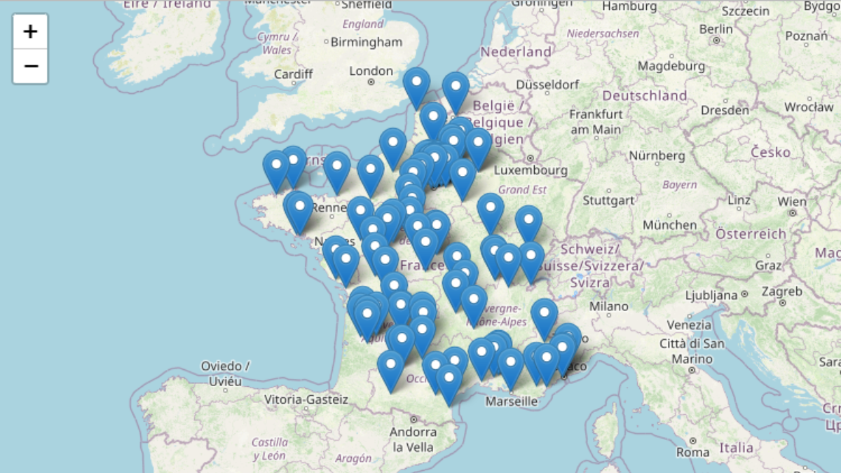
+ addMarkers(lng=monuments$longitude_num, lat=monuments$latitude_num)

addTiles() allows us to add the map tiles of the monuments, we will leave it empty for the moment.

addMarkers() is the essential point of our mapping since it contains the gps coordinates of the map markers via “lng (for longitude) and lat (for latitude).

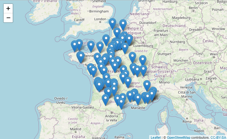
and here is the first result! Not bad, right?

Step 4: Add information to your markers

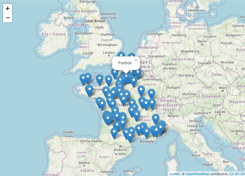
You can simply add information from your dataset to your markers and make your maps even more interactive with the popup. Our dataset has only the names of the monuments, so we will only include this information, but you could for example add several different lines/arguments.

carte_monuments <- monuments %>% 
leaflet() %>% 
addTiles() %>% 
addMarkers(lng=monuments$longitude_num, lat=monuments$latitude_num, popup = monuments$name)

and here is the rendering when clicking on a marker:

Step 6: Customize the card

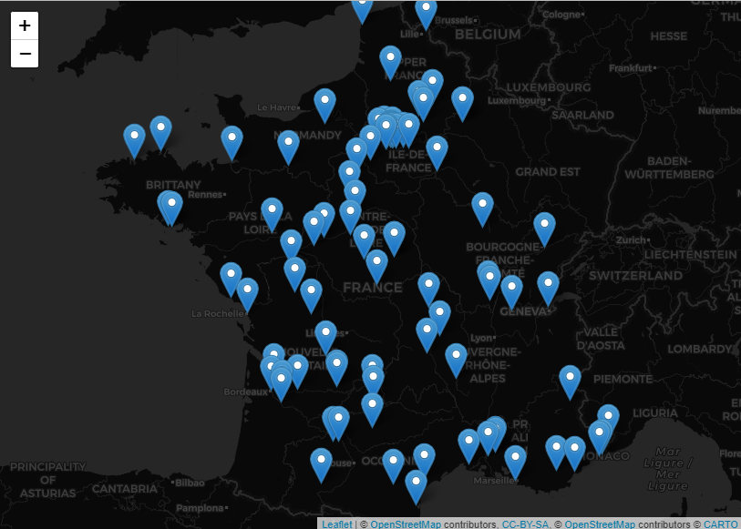
We can customize the map using CSS style sheets. For example, we can change the background color of the map using the addProviderTiles() function.

carte_monuments %>% 
  addProviderTiles("CartoDB.Positron") %>%
  addProviderTiles("CartoDB.DarkMatter")

The addProviderTiles() function adds tile layers for the map. We have added two layers: CartoDB.Positron for a light map and CartoDB.DarkMatter for a dark map. We can also use functions like addPolygons() to add polygons to the map, or addCircleMarkers() to add circle markers.

I hope this little guide will be useful to you in your learning of leaftlet(). Don’t forget to visit the leafletjs.com website to get precise information about the possibilities of the package.